3D plots with Plotly
‘plotly’ is a popular graphing package in Python, but also has an R interface. What makes plotly really cool is that it is by default interactive, which also makes it great for 3D plots. In this lesson we will make 3D plots in plotly.
Getting ready
First, let’s install the required packages for this tutorial plotly for plotting and reshape2 for making a best fit surface.
install.packages("plotly")
install.packages("reshape2")
Next we need to load up the packages.
library(plotly)
library(reshape2)
Loading up and checking the data
Then we load up and check our fake data
Data<-read.csv("Fake_data_3d_plots.csv")

str(Data)
## 'data.frame': 50 obs. of 4 variables:
## $ X : int 1 2 3 4 5 6 7 8 9 10 ...
## $ Growth_Rate: num 207.4 30.7 93 136.7 181.2 ...
## $ Density_1 : num 25.5 30.9 37.9 24.3 29.6 ...
## $ Density_2 : num 25.8 40.3 27.2 36.4 24.8 ...Our for data set has the density of 2 different species, and the growth rate for species 1.
Making the 3D scatter plot
The structure of plot_ly is similar to ggplot2. We first supply the name of data frame, and then map variables from our data frame to specific “aesthetics” (e.g., x-axis, y-axis, etc.). However, for plot_ly these are just separate parameters and not all within the aes() function. For this mapping we also need to use ~ in front of each variable.
To make a 3D scatter plot we need to specify an x-axis, y-axis, and z-axis. We also need to set type="scatter3d". Like ggplot2 we can save the plot as a variable to use later on. Finally the name parameter doesn’t show up, but is used to reference specific layers when customizing the plot (which we will use later).
p<-plot_ly(Data,x=~Density_1,y=~Density_2,z=~Growth_Rate,name="Data",type="scatter3d")

p
Plotly is interactive, so you can zoom in, zoom out, change the angle, and get information on specific data points.
Add predictions
Fit a model
Say we want to add predictions, so lets try to fit a model using lm with growth rate of species 1 as a function of density of species 1, density of species 2, and their interaction.
We use data argument to specify what data frame we are using, then put in the formula based on column names. Density_1:Density_2.
We can then use summary(model_1) to get information on the model we just fit.
model_1<-lm(data=Data,Growth_Rate ~ Density_1+Density_2+Density_1:Density_2)

summary(model_1)
##
## Call:
## lm(formula = Growth_Rate ~ Density_1 + Density_2 + Density_1:Density_2,
## data = Data)
##
## Residuals:
## Min 1Q Median 3Q Max
## -4.494 -1.696 0.242 1.490 3.764
##
## Coefficients:
## Estimate Std. Error t value Pr(>|t|)
## (Intercept) 396.78887 9.57549 41.438 <2e-16 ***
## Density_1 0.14535 0.31174 0.466 0.643
## Density_2 0.25639 0.32534 0.788 0.435
## Density_1:Density_2 -0.30577 0.01062 -28.781 <2e-16 ***
## ---
## Signif. codes: 0 '***' 0.001 '**' 0.01 '*' 0.05 '.' 0.1 ' ' 1
##
## Residual standard error: 2.102 on 46 degrees of freedom
## Multiple R-squared: 0.9992, Adjusted R-squared: 0.9991
## F-statistic: 1.905e+04 on 3 and 46 DF, p-value: < 2.2e-16Making Predictions
Next we can use the predict function to make predictions based on our model. The first argument is the saved model that we fit above, and the newdata argument is a data frame that has variables that match the variable names used to fit the model (in this case Density_1 and Density_2). The function will generate predictions at these these values. In this case we can supply the original data frame because we want to generate predictions of the model at the original data to visually see how well the model fits our data.
predictions<-predict(model_1, newdata = Data)
predictions
## 1 2 3 4 5 6 7 8
## 205.76162 30.26453 93.86870 138.82142 183.33419 217.30808 117.84127 104.46095
## 9 10 11 12 13 14 15 16
## -23.99789 67.16232 200.23285 -16.46752 180.61361 174.78481 23.73701 260.03999
## 17 18 19 20 21 22 23 24
## 196.53111 153.53361 83.52809 157.02114 95.07185 176.11158 69.93366 19.53620
## 25 26 27 28 29 30 31 32
## 135.82457 267.75781 49.23855 129.68867 44.59277 186.56241 50.26576 198.99010
## 33 34 35 36 37 38 39 40
## 113.24112 204.67605 254.03568 87.59822 232.06791 185.11934 174.48324 128.26608
## 41 42 43 44 45 46 47 48
## 84.30696 172.30643 216.79693 128.05856 180.18955 118.72169 64.66046 137.41530
## 49 50
## 178.34330 209.05358Adding predictions
Now we can add a new layer to the first 3D scatter plot that includes points of our predictions. We add new layers using %>%add_trace(...)
Like before we need to specify x, y, and z axes. Since we haven’t added the predictions (our z axis) to a dataframe we will put vectors into these arguments. Because they are vectors we don’t need to add the ~ like we did before.We will use the name parameter, for the legend (so it knows what to call this layer). marker=list(color="red") is how we specify the color of the predictions.
p_w_prediction<- p %>%add_trace(x = Data$Density_1, y = Data$Density_2, z =predictions , type = "scatter3d",name="Predictions_model_1",marker=list(color="red"))
p_w_prediction
## No scatter3d mode specifed:
## Setting the mode to markers
## Read more about this attribute -> https://plotly.com/r/reference/#scatter-mode
## No scatter3d mode specifed:
## Setting the mode to markers
## Read more about this attribute -> https://plotly.com/r/reference/#scatter-modePrediction surface
While it was cool to generate predictions at the same points we have data at, it’s probably more informative to generate predictions across the different combinations of densities. In a 2D scatter plot we can just use a line, but in 3D we need to make prediction surface/plane.
Make the prediction
First, we need to generate predictions across different possible combinations of the two density variables.
We will use the seq function which generates a vector of numbers in a sequence. The first argument is the minimum value, second argument is maximum value, and the third argument is the step of the sequence. To get those values, we will use the minimums and maximums of our density variables +/- 2 to give a little wider range for our surface.
SimD1 <- seq(min(Data$Density_1)-2,max(Data$Density_1)+2, 0.5)
SimD2<- seq(min(Data$Density_2)-2, max(Data$Density_2)+2, 0.5)
SimD1
## [1] 15.74147 16.24147 16.74147 17.24147 17.74147 18.24147 18.74147 19.24147
## [9] 19.74147 20.24147 20.74147 21.24147 21.74147 22.24147 22.74147 23.24147
## [17] 23.74147 24.24147 24.74147 25.24147 25.74147 26.24147 26.74147 27.24147
## [25] 27.74147 28.24147 28.74147 29.24147 29.74147 30.24147 30.74147 31.24147
## [33] 31.74147 32.24147 32.74147 33.24147 33.74147 34.24147 34.74147 35.24147
## [41] 35.74147 36.24147 36.74147 37.24147 37.74147 38.24147 38.74147 39.24147
## [49] 39.74147 40.24147 40.74147 41.24147 41.74147 42.24147SimD2## [1] 16.9604 17.4604 17.9604 18.4604 18.9604 19.4604 19.9604 20.4604 20.9604
## [10] 21.4604 21.9604 22.4604 22.9604 23.4604 23.9604 24.4604 24.9604 25.4604
## [19] 25.9604 26.4604 26.9604 27.4604 27.9604 28.4604 28.9604 29.4604 29.9604
## [28] 30.4604 30.9604 31.4604 31.9604 32.4604 32.9604 33.4604 33.9604 34.4604
## [37] 34.9604 35.4604 35.9604 36.4604 36.9604 37.4604 37.9604 38.4604 38.9604
## [46] 39.4604 39.9604 40.4604 40.9604 41.4604 41.9604Next, we need to get all possible combinations for these values. We can do that with the expand.grid. This creates a data frame with all possible combinations of the vectors we feed into the function. We can set the name of the columns in the result with =:
surface<- expand.grid(Density_1 = SimD1, Density_2= SimD2)
head(surface)
## Density_1 Density_2
## 1 15.74147 16.9604
## 2 16.24147 16.9604
## 3 16.74147 16.9604
## 4 17.24147 16.9604
## 5 17.74147 16.9604
## 6 18.24147 16.9604Now we can generate predictions like we did before with the predict function. Rather than save the results in a seperate vector, let’s just add a new column to the surface data frame:
surface$Growth_Rate<- predict(model_1, newdata = surface)
head(surface)
## Density_1 Density_2 Growth_Rate
## 1 15.74147 16.9604 321.7911
## 2 16.24147 16.9604 319.2708
## 3 16.74147 16.9604 316.7505
## 4 17.24147 16.9604 314.2302
## 5 17.74147 16.9604 311.7099
## 6 18.24147 16.9604 309.1896Unfortunately, to plot the prediction surface we need to format the data in a specific way, specifically matrix format. Where the rows are density 1, columns are density 2 and the numbers inside are the predictions. We can achieve this with the acast function from reshape2. This is how we use that function:
acast(data frame to transform, first predictor variable ~ second predictor variable, value.var = depednent variable column name)
surface_reshaped<-acast(surface, Density_1 ~ Density_2, value.var = "Growth_Rate")
surface_reshaped
## 16.9604011059768 17.4604011059768 17.9604011059768
## 15.7414680607694 321.7911 319.5126 317.2342
## 16.2414680607694 319.2708 316.9159 314.5610
## 16.7414680607694 316.7505 314.3192 311.8879
...Adding the surface
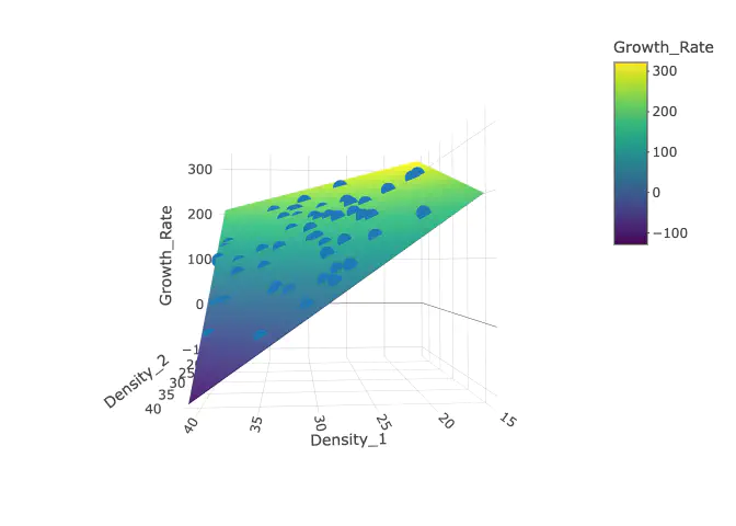
Next, let’s add the surface to the original plot. We put will supply the matrix into the z axis, and then the vectors that we used to create the prediction surface in the other axis columns. Finally we need to specify type="surface.
p_w_surface <- p %>% add_trace(x = SimD1, y = SimD2, z =surface_reshaped , type = "surface")
p_w_surface
## No scatter3d mode specifed:
## Setting the mode to markers
## Read more about this attribute -> https://plotly.com/r/reference/#scatter-modeTo make it look nicer, let’s just change the labels with the scene paramater in the layout() function.
p_w_surface %>% layout(scene = list(xaxis = list(title = 'Density 1'),
                                     yaxis = list(title = 'Density 2'),
                                     zaxis = list(title = 'Predicted Growth Rate')))
## No scatter3d mode specifed:
## Setting the mode to markers
## Read more about this attribute -> https://plotly.com/r/reference/#scatter-modeMatthew Kustra
Miller Postdoctoral Research Fellow
My research interests include sexual selection, speciation, and endosymbionts.